trialSizing

trialSizing provides tools for experimental design sizing in agricultural research: estimating the optimal plot size from a uniformity trial, and the number of replications needed to detect a given difference between treatments. Every method returns standardized diagnostic statistics and publication-style plots that can be saved to TIFF, PDF or PNG.

Cheat sheet

The whole package on one page, laid out in the order you actually use it. Click to open it full size — it is an SVG, so it stays sharp at any zoom and prints on one landscape sheet.

Installation

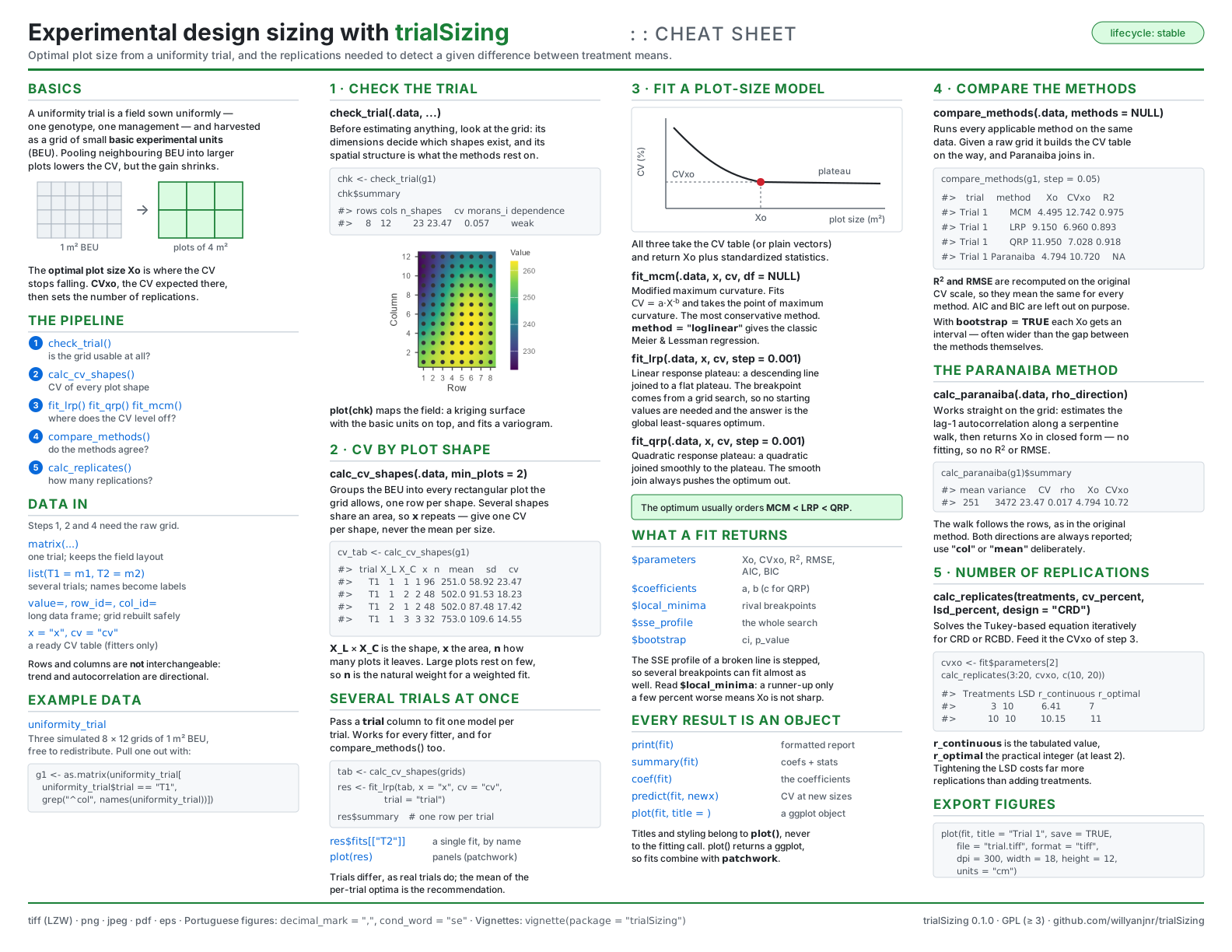
You can install the development version of trialSizing from GitHub with:

# install.packages("pak")
pak::pak("willyanjnr/trialSizing")

The workflow

A plot-size study starts from a uniformity trial -- a field sown uniformly and harvested in a fine grid of small basic experimental units (BEU) -- and walks through a fixed sequence of steps. trialSizing has one function for each:

Step	Question	Function
1	Is the grid usable, and how strong is the spatial structure?	check_trial()
2	What is the CV of every plot shape the grid allows?	calc_cv_shapes()
3	At what plot size does the CV stop falling?	fit_lrp(), fit_qrp(), fit_mcm()
4	How do the methods compare (incl. the closed-form Paranaiba)?	compare_methods(), calc_paranaiba()
5	Given that CV, how many replications are needed?	calc_replicates()

The rest of this page follows those steps on one dataset. Everything below uses uniformity_trial, a simulated trial bundled with the package (three 8 × 12 grids of 1 m² BEU; see ?uniformity_trial).

library(trialSizing)

# One trial, as the numeric grid the functions expect
grid1 <- as.matrix(uniformity_trial[uniformity_trial$trial == "T1",
                                    grep("^col", names(uniformity_trial))])
dim(grid1)   # 8 rows x 12 columns of 1 m^2 basic units
#> [1]  8 12

Step 1 — Check the trial

Before estimating anything, look at the raw grid: its dimensions decide which plot shapes exist at all, and its spatial autocorrelation is what the whole method rests on. check_trial() reports both, and plot() draws the field map.

chk <- check_trial(grid1)
#> Checking 1 trial(s).
chk
#> Uniformity trial check -- Trial 1 
#>   Grid:      8 x 12 = 96 basic units, 0 missing
#>   Shapes:    23 rectangular plot shapes available
#>   Values:    mean 251.013, sd 58.922, CV 23.47%, range [114.590, 368.440]
#>   Outliers:  0 by the boxplot rule
#>   Trend:     rows p = 0.387, columns p = 0.0336
#>   Moran's I: 0.057 (p = 0.367)   rho row 0.059, col 0.104
#>   Variogram: gaussian | nugget 3223.678, sill 3715.746, range 9.54
#>              nugget/sill 0.87 -> weak spatial dependence
#>              little spatial structure: plot size will buy little
#>              precision here, whatever method is used
#>   Issues:    none

Step 2 — CV by plot shape

calc_cv_shapes() groups the BEU into every rectangular plot the grid allows and returns one row per shape: the plot size x (in BEU), the number of plots n of that size, and the coefficient of variation cv among them. Several shapes share the same area, so x repeats.

cv_tab <- calc_cv_shapes(grid1)
#> CV by shape for 1 trial(s).
head(cv_tab)
#>     trial X_L X_C x  n      mean        sd       cv
#> 1 Trial 1   1   1 1 96  251.0129  58.92214 23.47375
#> 2 Trial 1   1   2 2 48  502.0258  91.52677 18.23149
#> 3 Trial 1   2   1 2 48  502.0258  87.47753 17.42491
#> 4 Trial 1   1   3 3 32  753.0388 109.57170 14.55061
#> 5 Trial 1   1   4 4 24 1004.0517 145.29792 14.47116
#> 6 Trial 1   2   2 4 24 1004.0517 135.13136 13.45861

This table is the input the plot-size models expect.

Step 3 — Fit a plot-size model

The CV falls steeply for small plots and then levels off; the plot size where it stops falling is the optimum. fit_lrp() finds it with a Linear Response Plateau model, by a grid search over the breakpoint (no starting values needed).

fit <- fit_lrp(cv_tab, x = "x", cv = "cv", step = 0.05)
#> Using x = 'x', cv = 'cv' (single series).
fit
#> Linear Response Plateau (LRP) fit
#> Method:                  segment  
#> Breakpoint (Xo):         9.150 
#> CV at breakpoint:        6.960 
#> R2: 0.893  RMSE: 1.513  AIC: 92.3  BIC: 96.9 
#> 
#> Local minima of the SSE profile (8):
#>   Xo =   7.400   SSE  +15.3% vs optimum
#>   Xo =  12.800   SSE  +34.5% vs optimum
#>   Xo =   5.750   SSE  +50.1% vs optimum
#>   ... see $local_minima for all

Title and styling belong to the plot() method, which draws the fitted broken line, the breakpoint and the plateau annotations:

plot(fit, title = "Uniformity trial T1")

plot of chunk fit-plot

To export a figure, use save = TRUE; TIFF is written with LZW compression, and vector formats are available for line art:

plot(fit, title = "Uniformity trial T1",
     save = TRUE, file = "trial.tiff", format = "tiff", dpi = 300)

Step 4 — Compare methods

The three CV-based models and the closed-form Paranaiba method often give different optima; the plot size typically increases in the order MCM < LRP < QRP. compare_methods() runs them all from a single grid (it builds the CV table on the way, and adds Paranaiba because it has the raw units):

compare_methods(grid1, step = 0.05)
#> Comparing 4 method(s) on 1 trial(s).
#> Plot-size methods compared
#> Trials: 1  | source: raw grid  | weighted: FALSE 
#> 
#>    trial    method     Xo   CVxo    R2  RMSE
#>  Trial 1       MCM  4.495 12.742 0.975 0.725
#>  Trial 1       LRP  9.150  6.960 0.893 1.513
#>  Trial 1       QRP 11.950  7.028 0.918 1.324
#>  Trial 1 Paranaiba  4.794 10.720    NA    NA
#> 
#> Xo ranges from 4.495 to 11.950 (a factor of 2.7).

calc_paranaiba() can also be called on its own; it works directly on the grid and returns a closed-form estimate from the first-order spatial autocorrelation:

calc_paranaiba(grid1)$summary
#> Paranaiba method on 1 trial(s); rho direction = 'row'.
#>     trial     mean variance       CV    rho_row    rho_col        rho       Xo
#> 1 Trial 1 251.0129 3471.819 23.47375 0.01655932 0.09052249 0.01655932 4.793933
#>       CVxo valid
#> 1 10.71956  TRUE

Because every plot() method returns a ggplot object, several fits can be shown side by side with patchwork:

library(patchwork)
lrp <- fit_lrp(cv_tab, x = "x", cv = "cv", step = 0.05)
qrp <- fit_qrp(cv_tab, x = "x", cv = "cv", step = 0.05)
mcm <- fit_mcm(cv_tab, x = "x", cv = "cv")

plot(mcm, title = "MCM", label_size = 3) +
  plot(lrp, title = "LRP", label_size = 3) +
  plot(qrp, title = "QRP", label_size = 3)

Several trials at once

Pass a data frame (or a list of grids) with a trial column to fit one model per trial. The result carries a per-trial summary table plus the individual fits (this works for fit_lrp(), fit_qrp(), fit_mcm() and compare_methods()):

grids <- lapply(split(uniformity_trial, uniformity_trial$trial),
                function(d) as.matrix(d[, grep("^col", names(d))]))

cv_all <- calc_cv_shapes(grids)
#> CV by shape for 3 trial(s).
res <- fit_lrp(cv_all, x = "x", cv = "cv", trial = "trial", step = 0.05)
#> Using x = 'x', cv = 'cv', trial = 'trial' -> 3 trials.
res$summary
#>   trial       a       b breakpoint plateau     R2   RMSE     AIC     BIC
#> 1    T1 21.0495 -1.5398       9.15  6.9602 0.8926 1.5131  92.322  96.864
#> 2    T2 19.3597 -1.0725      14.40  3.9162 0.8341 2.3486 112.547 117.089
#> 3    T3 21.3271 -1.5075      10.10  6.1011 0.8019 2.4138 113.806 118.348
#>   n_local
#> 1       8
#> 2       7
#> 3       8

Step 5 — Number of replications

The CV at the optimal plot size (CVxo) feeds directly into the number of replications needed to detect a given difference between treatment means (as a percent of the mean), for CRD or RCBD designs:

cvxo <- unname(fit$parameters["Breakpoint_Response"])

reps <- calc_replicates(
  treatments  = 3:20,
  cv_percent  = cvxo,
  lsd_percent = c(10, 20),
  design      = "CRD"
)
reps
#> Optimal number of replications
#> Design: CRD  CV: 6.96%  alpha: 0.05 
#> Rows: 36  | Non-converged: 0 
#> 
#>  Treatments CV_percent LSD_percent Alpha Design r_continuous r_optimal df_error
#>           3   6.960245          10  0.05    CRD         6.43         7       18
#>           4   6.960245          10  0.05    CRD         7.32         8       28
#>           5   6.960245          10  0.05    CRD         8.01         9       40
#>           6   6.960245          10  0.05    CRD         8.57         9       48
#>           7   6.960245          10  0.05    CRD         9.06        10       63
#>           8   6.960245          10  0.05    CRD         9.48        10       72
#>  q_tukey converged at_floor
#>    3.609      TRUE    FALSE
#>    3.861      TRUE    FALSE
#>    4.039      TRUE    FALSE
#>    4.197      TRUE    FALSE
#>    4.307      TRUE    FALSE
#>    4.415      TRUE    FALSE

The output reports both r_continuous (the tabulated value) and r_optimal (the practical integer, at least 2). Plotting shows how the requirement grows with the number of treatments, one line per LSD level:

plot(reps, title = "Replications needed")

plot of chunk replicates-plot

Where to go next

Each step has a dedicated vignette with the theory and the full set of options: vignette("check_trial"), vignette("cv_shapes"), vignette("lrp"), vignette("qrp"), vignette("mcm"), vignette("paranaiba"), vignette("compare") and vignette("replicates"). The methods are validated against published results in the tests and in vignette("validation").

Citation

If you use trialSizing in your research, please cite the underlying methods (see each function's documentation for the corresponding reference) as well as the package itself.